Hurst Exponent in Trading: Trend, Mean Reversion or Noise

The Hurst exponent (H) measures whether a market's returns tend to continue or reverse. H above 0.5 means persistent, trending behaviour; about 0.5 is a random walk; below 0.5 is mean-reverting. It is estimated as the slope of log rescaled range against log window size, and short samples need a bias correction.
A Hurst exponent of 0.58 looks like a trending market. On a few hundred bars it is usually just noise, because the classic estimator reads randomness as a mild trend. This Quantum Algo guide walks the rescaled-range method from Harold Hurst's Nile studies to a working regime filter: one chunk computed by hand, a full regression in numbers, the Anis-Lloyd correction, simulation results on how wide the error bars really are, and a calculator that gives you both the raw and corrected H for any price list.
Indicators that prove themselves in public.
One engine, four precision tools — the Gold (XAU) Scalper, the institutional Gravity Zone, the Zeno momentum Oscillator, and Zeno Stocks for equities.
From Nile floods to price charts: where the Hurst exponent comes from
Harold Edwin Hurst (1880–1978) was a British hydrologist who arrived in Egypt in 1906 and spent most of his long career studying the Nile. His practical problem was dam design: how big must a reservoir be so that it never runs dry in a drought and never overflows in a flood, given the river's erratic yearly flows?
If yearly flows were independent random draws, the answer follows from standard statistics, and the required storage grows with the square root of the time span. Hurst found that it didn't. In the Nile records, wet years tended to follow wet years and dry years followed dry years, so the cumulative surplus or deficit wandered further than independence allowed. He measured this with a statistic he called the rescaled range, published the method in "Long-Term Storage Capacity of Reservoirs" in the Transactions of the American Society of Civil Engineers (vol. 116, 1951, pp. 770–799), and his findings fed into the planning of the Aswan High Dam.
Benoit Mandelbrot later took the idea far beyond hydrology. With James Wallis he nicknamed long-run persistence the "Joseph effect", after the seven fat years and seven lean years of Genesis, and he carried the concept into finance as part of his fractal view of markets. That is how a statistic built for river levels ended up in trading software: the question "do wet years follow wet years?" becomes "do up-moves follow up-moves?"
What does the Hurst exponent actually measure?
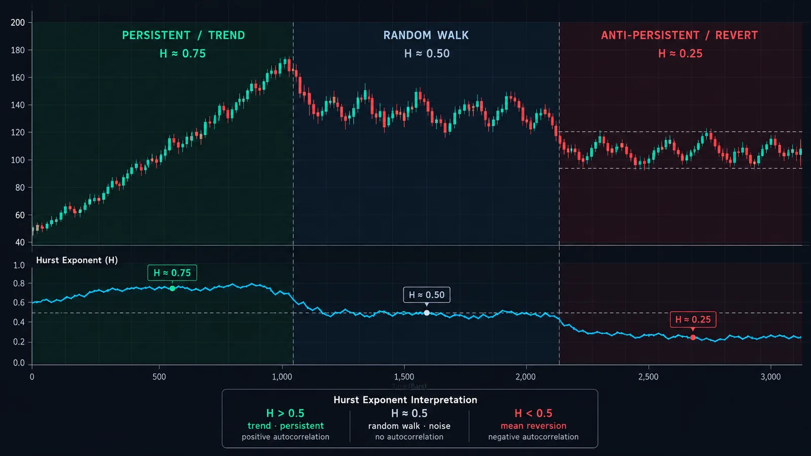
The Hurst exponent H describes how the spread of a cumulative series grows as you look at longer stretches of it. For a series of returns, it says how fast the range of the price path widens with time. The rescaled range scales roughly as a power law:
(R/S)ₙ ≈ c × nᴴ
where n is the window length. Take logs of both sides and H is simply the slope of a straight line through log(R/S) against log(n).
| H | Name | What it implies for returns | Strategies that fit |
|---|---|---|---|
| Below 0.5 | Anti-persistent | An up-move tends to be followed by a down-move; the path keeps folding back on itself | Mean reversion, fading oscillator extremes, range trading |
| About 0.5 | Random walk | Past moves carry no information about the direction of the next one | None based on direction alone |
| Above 0.5 | Persistent | Moves tend to continue; the path drifts away from where it started faster than chance | Trend following, channel breakouts, momentum |
Two points that most explanations skip.
H is about returns, not prices. You feed the estimator the changes (log returns), and it studies how their cumulative sum, which is the price path, spreads out. Feed raw price levels into the same procedure and you get nonsense: in our tests, running R/S on the price levels of a pure random walk returned H of about 0.99, which says only that prices are prices.
H is not about drift. The R/S calculation subtracts the average return of each window before doing anything else. A market grinding steadily higher with choppy, back-and-forth daily returns can have H below 0.5. In a simulation of 200 random walks with and without a strong upward drift of 0.4% per bar, the corrected H was identical to three decimals. A steady trend in the everyday sense and persistence in the Hurst sense are different things. The second one is what matters for whether a trend-following rule will work.
A related number you may see is the fractal dimension, D = 2 − H for a self-affine series. A rough, jagged mean-reverting chart has D near 2; a smooth persistent one has D closer to 1. It contains the same information as H.
How to calculate the Hurst exponent with R/S, step by step
The classical rescaled-range (R/S) estimator, as laid out in Hurst's work and in later reviews such as Weron's, runs like this on a series of L returns:
- Convert prices to log returns: rₜ = ln(Pₜ / Pₜ₋₁). Using logs keeps big and small price levels comparable.
- Pick window sizes. Choose several lengths n, usually doubling: 8, 16, 32, 64 and so on up to about L/2. Each needs at least two non-overlapping chunks.
- Split the series into L/n non-overlapping chunks of length n for each window size.
- Demean each chunk: subtract the chunk's average return from every return in it.
- Cumulate: build the running sum of the demeaned returns. This is the chunk's detrended price path.
- Range R: the maximum of the running sum minus the minimum.
- Scale S: the standard deviation of the chunk's returns.
- Rescale: compute R/S for the chunk, then average R/S across all chunks of the same length n.
- Regress: fit a straight line to log(average R/S) against log(n). The slope is the raw Hurst estimate.
- Correct for small-sample bias (optional but strongly recommended): subtract the R/S you would expect from pure noise at each n before fitting, then add 0.5. This is the Anis-Lloyd-Peters correction, covered below.
The calculator further down runs exactly these ten steps on any price list you paste, and reports both the raw and the corrected estimate.
Worked example: one chunk by hand, then the full regression
Step 1: R/S for a single 8-return chunk
Take eight returns, in percent: +1.0, +0.5, −0.8, +1.2, +0.3, −0.4, +0.9, +0.5. The units cancel out in R/S, so percent is fine.
| Return | Minus mean (0.4) | Running sum | Squared deviation |
|---|---|---|---|
| +1.0 | +0.6 | 0.6 | 0.36 |
| +0.5 | +0.1 | 0.7 | 0.01 |
| −0.8 | −1.2 | −0.5 | 1.44 |
| +1.2 | +0.8 | 0.3 | 0.64 |
| +0.3 | −0.1 | 0.2 | 0.01 |
| −0.4 | −0.8 | −0.6 | 0.64 |
| +0.9 | +0.5 | −0.1 | 0.25 |
| +0.5 | +0.1 | 0.0 | 0.01 |
The running sum peaks at 0.7 and bottoms at −0.6, so R = 1.3. The squared deviations total 3.36; divided by 8 that is 0.42, and the square root gives S = 0.648. So R/S = 1.3 / 0.648 = 2.006.
For comparison, the expected R/S of pure noise over 8 observations, from the Anis-Lloyd formula with Peters' adjustment, is 2.461. This chunk wandered less than noise would. One chunk tells you almost nothing, which is why the method averages many chunks and many window sizes.
Step 2: the regression across window sizes
Now a full run on 256 synthetic daily returns that we generated with mild short-term momentum (each day's return carries a quarter of the previous day's shock, an AR(1) process with φ = 0.25):
| Window n | Chunks | Average R/S | ln(n) | ln(R/S) | Expected R/S (noise) |
|---|---|---|---|---|---|
| 8 | 32 | 2.651 | 2.079 | 0.975 | 2.461 |
| 16 | 16 | 4.704 | 2.773 | 1.548 | 3.909 |
| 32 | 8 | 7.248 | 3.466 | 1.981 | 5.971 |
| 64 | 4 | 12.443 | 4.159 | 2.521 | 8.896 |
| 128 | 2 | 17.605 | 4.852 | 2.868 | 13.040 |
Fitting a least-squares line through the ln(n) and ln(R/S) columns gives a slope of 0.687. That is the raw Hurst exponent, and at face value it says "strongly trending".
Now fit the same line through the expected-noise column: its slope is 0.600. Pure randomness, measured over these particular windows, already produces a slope of 0.60, not 0.50. The corrected estimate is 0.5 + (0.687 − 0.600) = 0.587. Still persistent, but far less dramatic, and an honest reflection of the mild momentum we built in.
Notice one more thing. The process we simulated has only short memory: each return depends on yesterday and nothing further back. Yet it still pushes H above 0.5. This is exactly the problem Andrew Lo raised in 1991, and it matters for interpretation, as the research section explains.
Why raw R/S overstates H, and how the Anis-Lloyd correction fixes it
The classical R/S statistic is biased upward in short samples. Anis and Lloyd (1976, Biometrika 63(1): 111–116) derived the expected value of the rescaled range for independent normal observations, and Peters later added a small adjustment that improves it for very short windows. In the form Rafał Weron uses in his 2002 study of estimator accuracy:
E(R/S)ₙ = ((n − ½) / n) × Γ((n−1)/2) / (√π × Γ(n/2)) × Σᵢ₌₁ⁿ⁻¹ √((n − i) / i)
for n > 340, replace the gamma ratio with 1 / √(nπ/2)
The corrected Hurst exponent is 0.5 plus the slope of [log(R/S)ₙ − log E(R/S)ₙ] against log n. In words: measure how much faster than noise your series spreads, and add that to the noise baseline of 0.5.
How large is the bias in practice? We ran 200 simulated random walks (true H = 0.5) through the same estimator with windows starting at 8:
| Sample length (returns) | Raw R/S H (average) | Corrected H (average) | Spread of estimates (1 s.d.) |
|---|---|---|---|
| 128 | 0.575 | 0.457 | ±0.076 |
| 256 | 0.568 | 0.468 | ±0.055 |
| 512 | 0.558 | 0.473 | ±0.044 |
| 1,024 | 0.559 | 0.485 | ±0.034 |
Three conclusions.
- Uncorrected R/S reads a coin flip as a mild trend. A raw H of 0.57 on a few hundred bars is exactly what pure randomness produces. Weron found the same: classical R/S "overestimates the true Hurst exponent to a great extent".
- The corrected version slightly undershoots. It comes in a little below 0.5 on short samples, a small negative bias Weron also reported for the corrected R/S, DFA and periodogram estimators.
- The error bars are wide. With 256 returns, one standard deviation of the estimate is about 0.055. A reading of 0.54 is noise. Weron also showed that the popular rule-of-thumb significance band of ±1/√L is too narrow and flags false positives too often.
Weron's study used only windows longer than 50 for the corrected R/S, because including very short windows inflates the variance. That needs thousands of bars. Traders working with a few hundred bars will usually accept short windows, and should accept the wider error bars that come with them.
Alternatives to R/S: DFA, variance ratio and aggregated variance
R/S is the original, not the best. These are the estimators you will meet most often:
| Method | Idea | Strength | Weakness |
|---|---|---|---|
| Rescaled range (R/S) | Range of cumulative deviations over standard deviation, versus window size | Simple, historic, intuitive | Biased in small samples; sensitive to short-term autocorrelation |
| Detrended fluctuation analysis (DFA) | Fit a local trend line in each window of the cumulative series, measure the leftover fluctuation F(n), slope of log F versus log n | Most accurate on short samples in Weron's tests; tolerant of slow trends | More computation; no closed-form distribution |
| Variance ratio | Variance of q-bar returns divided by q times the 1-bar variance; above 1 means persistence, below 1 mean reversion | Has a formal test (Lo and MacKinlay, 1988) | Tests one horizon at a time |
| Aggregated variance | Variance of block averages shrinks like m^(2H−2) as block size m grows | Easy to compute | Noisy; confused by trends and level shifts |
| Periodogram (GPH) | Slope of the low-frequency end of the spectrum | Known asymptotic theory | Needs long samples |
DFA was introduced by Peng and colleagues in 1994 in a study of DNA sequences (Physical Review E 49: 1685–1689), and it is now the default in much of the physics and econophysics literature. Weron's comparison on simulated white noise called DFA "the unanimous winner" among the three methods he tested. If you are building your own regime filter and can afford the extra lines of code, use DFA and keep R/S as a cross-check. If your goal is a cleaner estimate of the underlying trend rather than a regime label, a state-space approach such as the Kalman filter answers that question more directly.
The variance ratio is worth knowing for a different reason. Lo and MacKinlay used it in "Stock Market Prices Do Not Follow Random Walks" (Review of Financial Studies, 1988) and strongly rejected the random walk for weekly US stock returns from 1962 to 1985, with the rejection driven largely by small stocks. It tests a specific horizon, which fits how traders think: "are 5-day moves persistent?" is a variance-ratio question.
Does the Hurst exponent work in markets? What the research says
The evidence is real but narrower than the trading-blog version.
- Short memory masquerading as long memory. Andrew Lo's "Long-Term Memory in Stock Market Prices" (Econometrica, 1991, 59(5): 1279–1313) built a modified R/S test that allows for short-range dependence. Applied to daily and monthly US stock indexes, it found no evidence of long-range dependence once short-term autocorrelation was accounted for, contrary to earlier claims based on classical R/S. Our worked example shows the mechanism: one day of momentum is enough to lift the classical estimate above 0.5.
- Hurst and predictability across markets. Eom, Choi, Oh and Jung studied 60 market indexes and found a strong positive relationship between each index's Hurst exponent and the hit rate of a nearest-neighbour forecast of price direction. Markets with higher H were more predictable, and the authors suggested the measure helps separate emerging from mature markets.
- Strategy switching. Chang, Lizardi and Shah (2022) used the Hurst exponent to choose between momentum and mean-reversion strategies and reported that the Hurst-based approach could achieve higher returns, though with higher risk.
- Estimator accuracy. Weron (2002) showed how wide the confidence intervals are on realistic sample sizes and that DFA is the most reliable of the common estimators.
Put together: daily returns of large, liquid markets sit close to 0.5, and apparent long memory often turns out to be short-term autocorrelation or volatility effects. That does not make H useless for traders. Short-term persistence is precisely what a trend-following rule exploits, and a measure that rises when it is present, and falls when returns start reversing, is useful even if an econometrician would not call it long memory. Just don't treat a reading of 0.58 as a discovery.
Using a rolling Hurst exponent as a regime filter
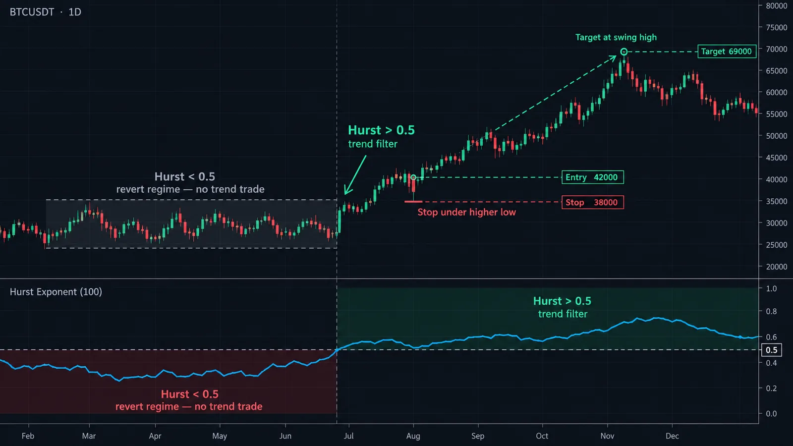
The most practical trading use is not forecasting price but choosing which kind of strategy to run. A rolling Hurst exponent, recalculated every bar on the most recent window of returns, acts as a switch between trend-following and mean-reversion playbooks.
A concrete design
- Window: 256 daily returns (about a year) on the instrument you trade, or 256 four-hour bars for a faster read. Shorter windows react quicker but the error bars widen fast.
- Estimator: corrected R/S or DFA, windows 8 to 128. Never the raw R/S slope, which is biased upward by about 0.07 at this length.
- Noise band: with 256 returns, readings within about ±0.05 of 0.5 are indistinguishable from randomness. A simple rule: band = 0.85 / √L, which is roughly one standard deviation in our simulations.
- Regimes: H above 0.55 = trend regime; below 0.45 = mean-reversion regime; anything between = stand aside or trade smaller.
- Hysteresis: enter a regime when H crosses the band edge, exit only when it crosses back through 0.5. That stops the switch from flickering every few bars.
- Smoothing: a short average (5 to 10 bars) of the rolling H reduces noise further, at the cost of a few bars' delay.
What runs in each regime
- Trend regime: breakouts and moving-average systems such as an ALMA crossover or a McGinley Dynamic trend line, with trailing exits.
- Mean-reversion regime: fades of band extremes using Bollinger Bands or RSI extremes, with fixed targets near the mean. Our mean reversion trading guide covers rules for this side.
- Neutral: reduced size, or nothing.
The same idea works for pairs and spreads. A spread with a persistently low Hurst exponent is a candidate for mean-reversion trading; one whose H climbs toward 0.5 or above is losing the property that made it tradable.
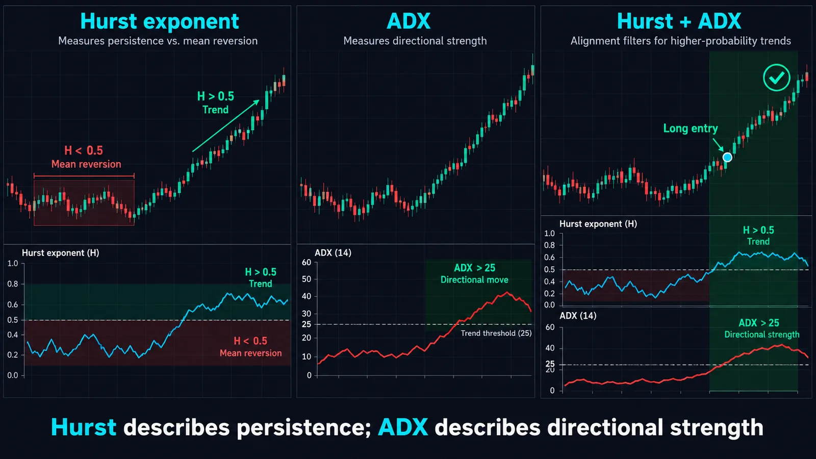
If you'd like a second opinion that doesn't rely on return statistics, the ADX measures trend strength from price ranges and makes a useful cross-check; the two often disagree at turning points, which is information in itself.
Is there a Hurst exponent indicator on TradingView?
TradingView does not include a Hurst exponent among its built-in indicators, as far as we can find. The community library has a number of open-source scripts that estimate it, usually plotted as an oscillator in a separate pane with a 0.5 reference line. Search "Hurst" in the Indicators dialog and filter to Community scripts.
Before you trust any of them, open the source code and check five things:
- Returns or prices? The estimator must run on returns (ideally log returns). A script that feeds price levels into R/S will sit near 1.0 forever.
- Raw or corrected? If the script fits log(R/S) without subtracting the expected noise value, subtract roughly 0.05 to 0.10 from its readings in your head on typical lookbacks.
- Window sizes. At least three or four sizes should go into the regression. A "Hurst" computed from a single window is just a scaled range, not an exponent.
- Lookback. Under about 100 bars, the estimate is too noisy to separate 0.45 from 0.55 reliably.
- Repainting. A proper rolling estimate only uses closed bars. If historical values shift when you reload the chart, see our non-repaint indicators guide.
A practical note for Pine authors: R/S across several window sizes on every bar involves nested loops, which can hit Pine's execution limits on long lookbacks. Compute it only on the last bar or every N bars if you just need the current regime. For the platform basics, see our TradingView platform guide. To sanity-check any script, export or copy a few hundred closes into the calculator on this page and compare.
Common mistakes and when the Hurst exponent misleads
- Reading raw R/S at face value. On a few hundred bars, raw R/S averages about 0.57 on pure noise. Use the corrected version or DFA.
- Ignoring the error bars. With 256 returns, ±0.055 is one standard deviation. Regime calls inside 0.45 to 0.55 are guesses.
- Confusing short and long memory. One day of momentum lifts H. That may be tradable, but it decays quickly; don't extrapolate it to multi-month horizons.
- Non-stationary samples. A window that contains a crash and a calm recovery mixes two regimes. Volatility clustering itself had little effect in our simulations, but structural breaks, such as a policy change, a halving cycle in crypto, or a product rolling from one contract to another, can distort the estimate badly. Use back-adjusted continuous contracts for futures.
- Mixing timeframes. H on 5-minute returns and H on daily returns answer different questions and can point opposite ways, so measure it on the timeframe you actually trade, whether that is daily swings or scalping charts. Microstructure effects such as the bid-ask bounce push very short-timeframe returns toward mean reversion.
- Calling drift persistence. A strong uptrend with choppy returns can read 0.5 or lower. If you need a trend-in-price measure, use slope-based tools such as a linear regression channel alongside H.
- Optimizing the threshold. Choosing 0.53 because it maximized a backtest is data snooping. Set the band from sample size, not from results.
- Too few window sizes. Two points always fit a line perfectly. Use at least three, preferably four or more.
Hurst Exponent and Quantum Algo
The Hurst exponent answers a question most indicators never ask: is this market currently rewarding trend-following or fading? That makes it a filter, not a trigger. It tells you which tools to pick up, not when to press the button.
A workable division of labour: a rolling, corrected Hurst on your instrument sets the regime; in the trend regime, signal tools take over the timing. With QuantumAlgo's Zeno suite, that means taking Zeno's buy and sell signals, which come with built-in stops and targets, more readily when the regime reads persistent and standing aside or sizing down when it reads anti-persistent. You can judge the signals on their own merits on the public track record. In mean-reversion regimes, our free Market Bottom Finder and Multi-Oscillator Divergence Scanner are closer to the job, and the Event Probability Engine suits traders who already think in probabilities.
For the statistical side, the related machine learning indicators guide covers other ways to classify market state, and the free Academy builds up the trend and mean-reversion foundations both regimes depend on.
◆ Interactive check
How well do you know the Hurst exponent?
Questions traders ask about the Hurst exponent
It is a number between 0 and 1 that describes whether returns tend to continue or reverse. Above 0.5 suggests trending behaviour, around 0.5 a random walk, and below 0.5 mean reversion. Traders mainly use it to decide which kind of strategy suits current conditions.
The classic method is rescaled range analysis: split log returns into chunks of several sizes, compute the range of cumulative deviations divided by the standard deviation for each chunk, average by size, and take the slope of log(R/S) against log(size). Correct the result against the expected R/S of noise on short samples.
There is no good or bad value, only fit. Trend strategies want readings clearly above 0.5 and mean-reversion strategies want readings clearly below it. With a few hundred bars, anything between about 0.45 and 0.55 should be treated as random.
British hydrologist Harold Edwin Hurst, while studying Nile river flows to size reservoirs. He published the rescaled range method in 1951. Benoit Mandelbrot later extended the idea and applied it to financial markets.
It means the returns behave like a random walk: past direction says nothing about future direction. On short samples, an uncorrected estimate of 0.55 to 0.58 can also be consistent with a random walk because of bias.
At least a few hundred returns for a usable trading estimate, and thousands for research-grade precision. With 256 returns, one standard deviation of the estimate is around 0.05 in our simulations.
Usually yes. In Weron's 2002 comparison on simulated data, detrended fluctuation analysis was the most accurate of the methods tested. R/S remains useful as a simple cross-check.
There is no built-in one as far as we can find, but several community scripts estimate it. Check that a script uses returns, applies a bias correction and regresses over several window sizes before trusting it.
No. It describes the character of recent returns, not which way the next move goes. Research such as Eom and colleagues' study of 60 indexes links higher H to better predictability, but direction still has to come from your strategy.
It is the expected rescaled range of independent normal data, derived by Anis and Lloyd in 1976 and refined by Peters. Subtracting it from the observed R/S at each window size removes most of the upward bias of the classic estimator.
References & Related Guides
Read next
- Mean Reversion Trading
- ADX Indicator (Average Directional Index)
- Machine Learning Trading Indicators
- Bollinger Bands
- Linear Regression Channel
- Kaufman Adaptive Moving Average (KAMA)
- Williams %R
- Donchian Channels
- Kalman Filter Trading
- ALMA Indicator
- Free TradingView indicators
- Zeno — the premium engine
Primary sources
- Wikipedia — Hurst exponent
- Wikipedia — Harold Edwin Hurst
- Weron (2002) — Estimating long range dependence: finite sample properties and confidence intervals (arXiv)
- Econometric Society — Lo (1991), Long-Term Memory in Stock Market Prices, Econometrica 59(5)
- MIT — Lo & MacKinlay (1988), Stock Market Prices Do Not Follow Random Walks
- Eom, Choi, Oh & Jung — Hurst exponent and prediction based on weak-form efficient market hypothesis (arXiv)
- Chang, Lizardi & Shah (2022) — Optimizing Returns Using the Hurst Exponent and Q Learning (arXiv)
- Wikipedia — Detrended fluctuation analysis