Kalman Filter Trading: How the Indicator Works and When It Helps
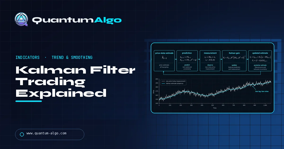
A Kalman filter in trading is a recursive smoother that estimates the true price level by blending its own prediction with each new bar, weighted by a gain set from process noise Q and measurement noise R. The simple one-state version settles into an EMA; lower lag comes only from adding a velocity state or adaptive noise settings.
Kalman filter indicators are sold as "zero-lag" moving averages. Run the math and a different picture appears: the common one-dimensional version settles into an ordinary EMA whose length you can calculate from two inputs. This Quantum Algo guide shows that calculation, works five bars by hand, explains where genuinely lower lag comes from (a velocity state, adaptive noise), and covers the use where Kalman filters have the best published record: time-varying hedge ratios for pairs trading. There is also a calculator so you can test your own prices.
Indicators that prove themselves in public.
One engine, four precision tools — the Gold (XAU) Scalper, the institutional Gravity Zone, the Zeno momentum Oscillator, and Zeno Stocks for equities.
Why traders put a Kalman filter on a price chart
Every price print is a mix of two things: where the market "really" is, and noise from the order book, spreads and impatient traders. A moving average tries to separate the two by averaging a fixed window. A Kalman filter does it differently. It keeps a running best guess of the true level, keeps a number for how uncertain that guess is, and when a new bar arrives it decides how much to believe the bar versus its own guess.
That decision is the whole trick. If the filter is unsure of itself and prices are clean, it follows price closely. If it is confident and prices are noisy, it barely moves. The weight it gives each new bar is called the Kalman gain, and it is recalculated on every bar.
The method comes from engineering, not markets. Rudolf E. Kálmán published "A New Approach to Linear Filtering and Prediction Problems" in the Journal of Basic Engineering in 1960, and an early implementation by Stanley Schmidt's team at NASA Ames ended up in the Apollo navigation computer. Traders borrowed it for three jobs:
- A smoothed trend line that you read like a moving average.
- A trend-plus-slope estimate that projects momentum forward to cut lag.
- A time-varying hedge ratio for pairs and spread trading, which is where it has the strongest track record in published quant work.
Most articles stop at "it adapts, so it is better." The useful truth is more specific, and it starts with the equations.
The Kalman filter equations, one line at a time
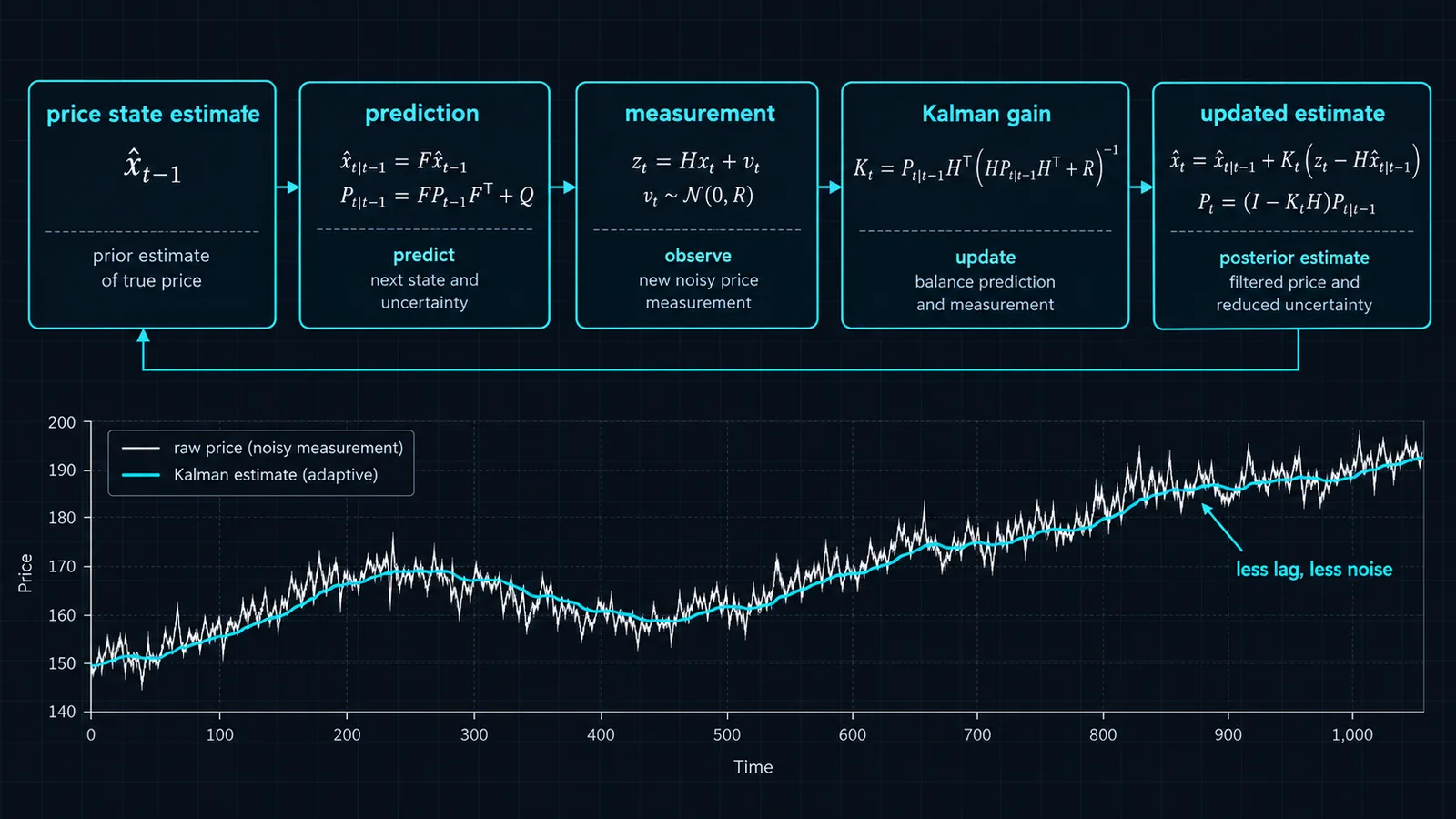
For price smoothing, traders almost always use the simplest version: one hidden state (the true price level) that is assumed to wander like a random walk. Statisticians call this the local level model. Each bar runs two phases, predict and update.
Predict: x⁻ = x(t−1) P⁻ = P(t−1) + QGain: K = P⁻ ÷ (P⁻ + R)Update: x(t) = x⁻ + K × (price − x⁻) P(t) = (1 − K) × P⁻| Symbol | Name | What it means on a chart |
|---|---|---|
| x | State estimate | The filter line you plot |
| P | Estimate variance | How unsure the filter is about its own line |
| Q | Process noise | How much you think the true level really moves per bar |
| R | Measurement noise | How noisy you think each price print is |
| K | Kalman gain (0 to 1) | The share of the latest surprise that gets added to the line |
Read the update line slowly: new estimate equals old estimate plus K times the surprise. That is exactly the shape of an exponential moving average, where the EMA adds α times the surprise. The only difference is that the EMA's α is fixed by you, while K is computed from P, Q and R.
The general filter uses matrices (a transition matrix F, an observation matrix H, and covariance matrices for Q and R) so it can track several hidden values at once. The one-dimensional version above is the special case where everything is a single number.
How Q and R trade smoothness for responsiveness
Here is the fact that most Kalman indicator pages bury: in the one-dimensional model, the gain settles to a fixed value after a few dozen bars, and that value depends only on the ratio q = Q ÷ R. Scale both by ten and nothing changes.
Steady-state gain: K∞ = ( −q + √(q² + 4q) ) ÷ 2, where q = Q ÷ REquivalent EMA length: N = 2 ÷ K∞ − 1Once K has settled, the filter is mathematically identical to an EMA with α = K∞. The textbook Forecasting: Principles and Practice shows the same link from the other side: simple exponential smoothing can be written as an innovations state-space model whose state equation is level(t) = level(t−1) + α × error.
| q = Q ÷ R | Steady-state gain K∞ | Behaves like EMA of | Character |
|---|---|---|---|
| 0.001 | 0.031 | ≈ 63 bars | Very smooth, slow |
| 0.01 | 0.095 | ≈ 20 bars | Swing-trend baseline |
| 0.05 | 0.200 | 9 bars | Short-term trend |
| 0.1 | 0.270 | ≈ 6.4 bars | Fast |
| 0.5 | 0.500 | 3 bars | Hugs price |
| 1.0 | 0.618 | ≈ 2.2 bars | Almost raw price |
This table is the most practical thing in this guide. One widely used open-source TradingView Kalman script defaults to Q = 0.01 and R = 0.1, a ratio of 0.1. In steady state that line carries the same weighting as roughly a 6-period EMA. Knowing that, you can stop guessing what a setting does and match it to an average you already understand.
A five-bar Kalman filter, computed by hand
Let us run the filter on six closes: 100.00, 101.20, 100.60, 102.10, 103.00, 102.40. Settings: Q = 0.1, R = 1, starting estimate x = 100.00 (the first close) and starting variance P = 1.
| Bar | Close | P⁻ = P + Q | Gain K | Estimate x | New P |
|---|---|---|---|---|---|
| 1 | 101.20 | 1.1000 | 0.5238 | 100.6286 | 0.5238 |
| 2 | 100.60 | 0.6238 | 0.3842 | 100.6176 | 0.3842 |
| 3 | 102.10 | 0.4842 | 0.3262 | 101.1012 | 0.3262 |
| 4 | 103.00 | 0.4262 | 0.2988 | 101.6686 | 0.2988 |
| 5 | 102.40 | 0.3988 | 0.2851 | 101.8772 | 0.2851 |
Bar 1 in full
- Predict: x⁻ = 100.00, P⁻ = 1 + 0.1 = 1.1.
- Gain: K = 1.1 ÷ (1.1 + 1) = 0.5238.
- Surprise: 101.20 − 100.00 = 1.20.
- Update: x = 100.00 + 0.5238 × 1.20 = 100.6286.
- New variance: P = (1 − 0.5238) × 1.1 = 0.5238.
What the numbers show
The gain falls every bar: 0.52, 0.38, 0.33, 0.30, 0.29. It is heading for the steady-state value of 0.270 from the table above. While it is high, the filter chases price harder than its steady-state EMA would. An EMA with α fixed at 0.270 on the same data ends bar 5 at 101.697; the Kalman line ends at 101.877, closer to price, purely because of that warm-up.
Now the uncomfortable comparison. A plain 5-period EMA (α = 0.333) seeded at 100 ends bar 5 at 101.916, even closer to price than the Kalman line. So "Kalman is faster than an EMA" depends entirely on which EMA and which Q/R you compare. Paste these closes into the calculator below to check every number.
Choosing Q and R for your market and timeframe
Here is something that surprises most people who read Kalman code for the first time: in the classic linear filter, the gain sequence never looks at prices. P, P⁻ and K depend only on Q, R and the starting P. You could compute every gain before the chart even loads. Prices only enter through the surprise term. That is why the Q ÷ R ratio, not the instrument, decides the behavior, and why a script with fixed Q and R behaves the same on Bitcoin as on EUR/USD.
The starting variance P does matter for the first few dozen bars. A P that is large relative to R makes the line jump to price at the start; a tiny P makes it crawl. Setting the starting estimate to the first close and P equal to R is a neutral choice.
Starting points, not magic numbers
These are reasonable first settings expressed as q = Q ÷ R, chosen to match moving-average lengths traders commonly use on each horizon. They are a place to begin testing, not optimized values.
| Use | Typical timeframe | Starting q | Behaves like |
|---|---|---|---|
| Scalping baseline | 1 to 5 minute | 0.05 to 0.1 | EMA 6 to 9 |
| Intraday trend | 15 minute to 1 hour | 0.01 | EMA 20 |
| Swing bias | 4 hour to daily | 0.002 to 0.005 | EMA 28 to 45 |
| Position trend | Daily to weekly | 0.0005 to 0.001 | EMA 63 to 89 |
Estimating Q and R from data
If you want something more principled than matching an EMA, estimate the two noises directly. R is the variance of prices around their underlying level: take a smooth reference line, compute close minus line for each bar, and use the variance of that residual. Q is the variance of bar-to-bar changes in the reference line itself. On a liquid index future in a calm week, that usually produces a small q; in a news-driven week it jumps. Statisticians fit these by maximum likelihood instead, which is what the state-space tools in Python and R do, but the residual method gets you within the right order of magnitude.
Whatever method you use, recheck after a volatility shift. A ratio estimated in a quiet regime is the single most common reason a Kalman line that looked perfect last month is lagging badly this month.
Does a Kalman filter really lag less than an EMA?
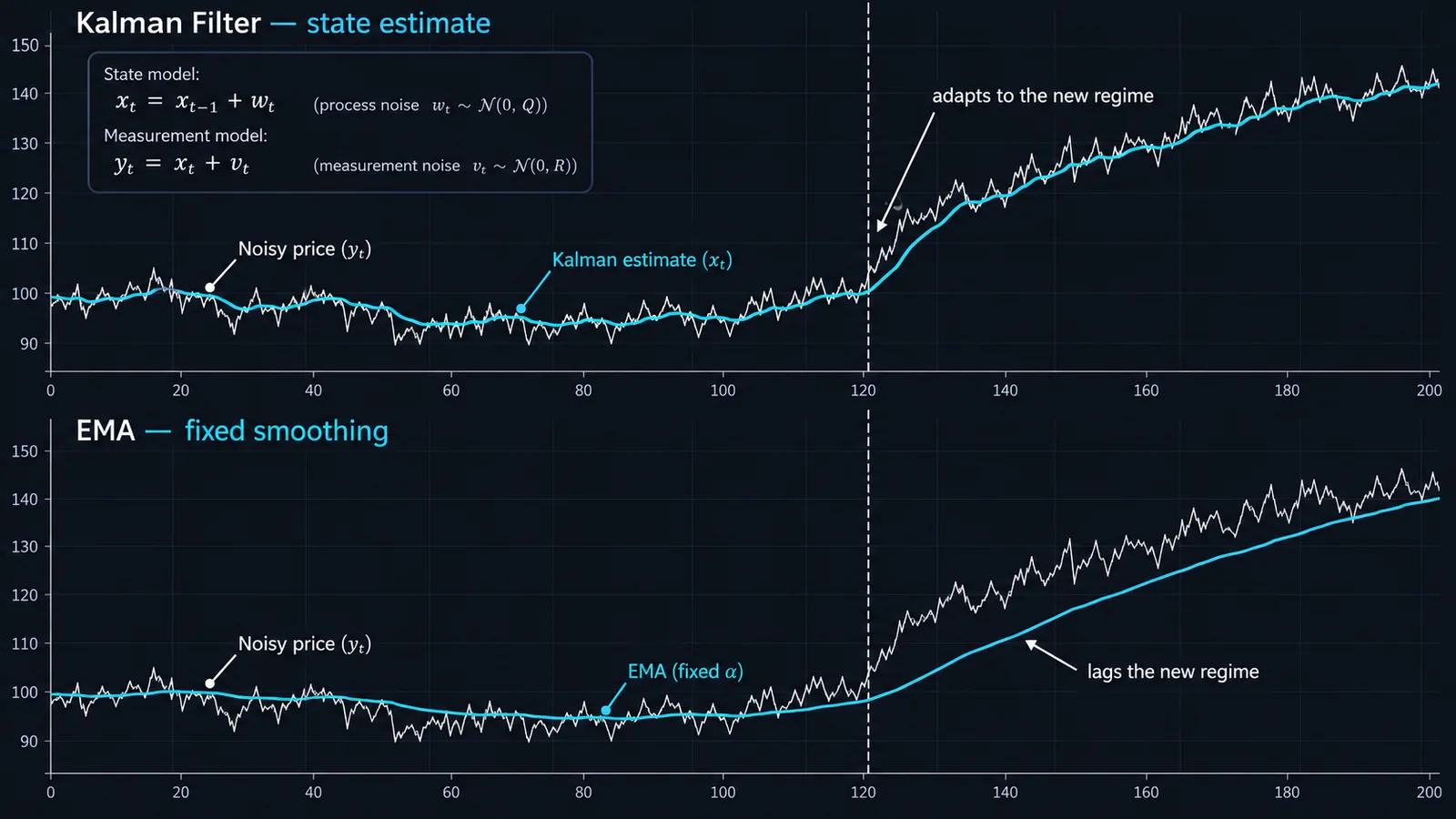
Short answer: the one-dimensional level filter does not, once it has warmed up. It lags exactly like the EMA it converges to. Claims of lower lag come from three other places, and each has a price.
- Warm-up and resets. A high starting P makes the early gain large, so the line snaps to price at the start of the chart. Some scripts inflate P after big moves to get the same effect mid-chart. That reduces lag right after shocks and increases noise right after shocks.
- Adaptive Q and R. Scripts that scale R or Q with ATR or standard deviation change the gain with volatility. That is closer in spirit to Kaufman's adaptive moving average than to a classic Kalman filter, and it adds parameters you have to tune.
- A velocity state. This is the real one. If the model tracks level and slope, the prediction step projects the trend forward, so the line keeps up in a steady trend. It also overshoots at turns, the same trade-off you see with the Hull moving average.
None of this is free lunch. Lower lag in trends always shows up as more overshoot and more whipsaw somewhere else. What the Kalman framework buys you is a principled way to set that trade-off, plus an uncertainty band (from P) that a moving average does not give you.
The two-state version: level plus velocity
The constant-velocity model adds a second hidden value, the slope per bar. The prediction step becomes "next level = level + slope; next slope = slope." Only the level is observed, so the filter infers the slope from how prices keep surprising it.
State: [level, slope] F = [[1, 1], [0, 1]] H = [1, 0]Predict: level⁻ = level + slope, slope⁻ = slope, P⁻ = F·P·Fᵀ + QIn practice this behaves like a smoothed linear projection, similar in feel to a rolling linear regression line but updated recursively. The slope state is useful by itself: plot it as an oscillator and it becomes a smoothed rate-of-change that crosses zero when the trend flips.
Eric Benhamou's 2016 paper "Trend Without Hiccups: A Kalman Filter Approach" compared several such models with DEMA and TEMA on one year of daily E-mini S&P 500 data. The models were tuned on that same year with no out-of-sample test, so treat the reported profits as a demonstration, not evidence of an edge.
Kalman hedge ratios in pairs trading
This is where the Kalman filter earns its reputation. In a pairs trade you hold one asset against another in a ratio β so that the spread is mean-reverting. A fixed β from one regression goes stale; a rolling regression forces you to pick a lookback. The Kalman approach treats β (and an intercept) as hidden states that drift as a random walk, and updates them every bar.
Observation: priceY(t) = β₀(t) + β₁(t) × priceX(t) + noiseState: β(t) = β(t−1) + small random changeErnest Chan popularized the method for retail quants in Algorithmic Trading: Winning Strategies and Their Rationale (Wiley, 2013), using the EWA and EWC country ETFs. The filter also gives you two by-products: the forecast error e(t), which is the spread, and its variance, whose square root works like a moving standard deviation. Trade it like Bollinger Bands on the spread: go long the spread when e(t) falls below −k × √variance, short when it rises above +k × √variance.
QuantStart's write-ups apply the method to the TLT and IEI Treasury ETFs. In its QSTrader backtest (daily bars, August 2009 to August 2016, threshold of one standard deviation) the article reports a CAGR of 8.73%, a Sharpe ratio of 0.75 and a 15.79% maximum drawdown, explicitly gross of transaction costs, with a 777-day drawdown duration. That last number is the honest one: even a textbook-good pairs filter can go two years without a new equity high. For the broader logic of fading stretched spreads, see our mean reversion trading guide.
Setting up a Kalman filter indicator on TradingView
TradingView has no built-in Kalman filter, so you will be using a community script. Search "Kalman" in the Indicators dialog and you will find dozens: plain level filters, adaptive versions that scale with ATR, Kalman-smoothed RSI and oscillator variants. Before adding one, check four things in the description or source:
- Which model. One state (level) or two (level and velocity)? A one-state script will behave like an EMA once warmed up.
- Which inputs. Separate Q and R, or a single "smoothness" input? If separate, compute q = Q ÷ R and look it up in the table above.
- Adaptive scaling. If Q or R is multiplied by ATR or standard deviation, the line will change character between quiet and volatile sessions. Our ATR guide explains what that volatility input measures.
- Repainting. A forward filter that only uses past bars does not repaint. A Kalman smoother (which runs backward over the data) does, and it will look magical on historical charts. Our guide to non-repainting indicators shows how to test this with bar replay.
A practical tuning routine
- Pick the EMA length you already trust on that market and timeframe, say 20 on a 1-hour chart.
- Convert it: α = 2 ÷ 21 = 0.095. That corresponds to q ≈ 0.01, so start with Q = 0.01 and R = 1.
- Overlay both lines. They should nearly coincide after the warm-up. If they do, the script is a level filter and you now know its baseline.
- Only then experiment: adaptive scaling, a velocity state, or a different q. Change one thing at a time and judge on out-of-sample bars.
If scripts and inputs are new to you, our TradingView platform guide covers adding, saving and templating indicators.
Kalman filter vs EMA, ALMA and McGinley Dynamic
All of these try to answer the same question: how much should the line move on this bar? They answer it with different machinery.
| Smoother | How it sets its speed | Lag in a steady trend | Main risk |
|---|---|---|---|
| EMA | Fixed α = 2 ÷ (N + 1) | Moderate, constant | Too slow or too noisy, never both right |
| Kalman (level) | Gain from Q, R and P; settles to a fixed value | Same as its equivalent EMA once warmed up | Mistaking warm-up speed for an edge |
| Kalman (level + velocity) | Gain plus slope projection | Low | Overshoot at turning points |
| ALMA | Gaussian weights shifted toward recent bars (offset, sigma) | Low to moderate | Offset set too high gets jumpy |
| McGinley Dynamic | Speed adjusts with the ratio of price to the line | Moderate, catches up faster in sell-offs | Can trail in sharp rallies |
| KAMA | Efficiency ratio of direction vs noise | Low in clean trends, flat in chop | Slow to restart after a range |
If you want a filter that also tells you how wide the noise band is, Kalman wins: P gives you an uncertainty estimate for free. If you just want a line, an ALMA or a well-chosen EMA is simpler to reason about. For a channel-style alternative built on a different smoothing family, see the Gaussian Channel guide.
Where Kalman filters fail in live trading
- Regime changes. Q and R are guesses about how much the market moves and how noisy it is. A Q tuned on a quiet month will lag badly in a news-driven trend; one tuned on a trending month will whipsaw in a range. Checking whether the market is trending or mean-reverting first, for example with the Hurst exponent, tells you which regime you are tuning for.
- Overfitting. With adaptive multipliers, velocity noise, initial P and a signal threshold, a "simple" Kalman system easily has five or six free parameters. Optimize them on one sample and the backtest will look clean. Hold back at least a third of your data and test once.
- Fat tails. The filter assumes Gaussian noise. One gap or flash spike creates a huge surprise, and the line jumps by K times that surprise. Clip extreme surprises or filter on a steadier input such as the bar's median price.
- Broken pairs. In pairs trading, the filter will keep updating β even when the relationship has truly ended. It adapts to a broken spread instead of warning you. Pair it with a periodic cointegration check.
- The smoother trap. Backward-looking Kalman smoothers use future bars. Any backtest built on them is invalid.
- Crossover systems. Price crossing a Kalman line whipsaws exactly as much as price crossing the equivalent EMA. Changing the name of the average does not fix crossover noise; filters like a Supertrend band or a volatility buffer do.
Three sensible ways to use a Kalman line
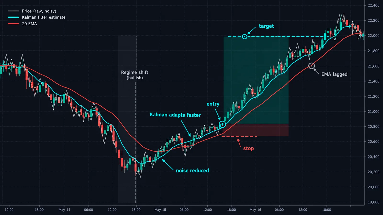
- Trend bias. Use a slow setting (q around 0.001 to 0.01) as a bias line. Above and rising, look for longs; below and falling, look for shorts. Same job as a 50-period average, with a P-based band to show how far price can stray before the bias is in doubt.
- Slope oscillator. With the two-state model, plot the velocity state. Zero crosses mark trend flips with less noise than a raw momentum oscillator, similar in spirit to the MACD histogram.
- Spread z-score. For pairs or for price vs its own Kalman line, divide the surprise by √P⁻ (or by the forecast-error standard deviation). That gives a self-scaling z-score for mean-reversion entries.
Kalman filters also show up as preprocessing inside more complex models. If that direction interests you, our guide to machine learning trading indicators covers how smoothed inputs feed classifiers.
Kalman Filter and Quantum Algo
A Kalman line is a good answer to "which way is the trend and how noisy is it?" It is not an entry system. That split maps cleanly onto how we build tools at Quantum Algo. Use a slow Kalman setting as a directional filter, then let a timing tool handle entries and risk. Zeno's signals come with a stop and targets built in, so the Kalman bias decides which side you are allowed to take, and Zeno decides when and where the risk is defined. On gold, Zeno Gold works across timeframes; on index CFDs, Zeno Stocks covers NAS100 and SPX500.
If you would rather stay free and open-source, the Adaptive Trend Sentinel is an adaptive trend line you can compare side by side with a Kalman script, and the Supertrend Engine adds a volatility buffer to cut crossover whipsaw. All QuantumAlgo free scripts are on the free indicators page, and the Academy covers trend filters from first principles.
◆ Interactive check
How well do you know Kalman filters?
Questions traders ask about Kalman filters
It is a recursive estimator that tracks a hidden value, usually the true price level or a hedge ratio, from noisy prices. Each bar it predicts, measures the surprise, and corrects by a gain that depends on process noise Q and measurement noise R.
Not automatically. The one-state Kalman filter converges to an EMA, so after warm-up it lags the same. Its advantages are an uncertainty estimate and the option to add a velocity state or time-varying parameters. Compare with our moving averages guide.
Only the ratio Q ÷ R matters in the simple model. A ratio near 0.01 behaves like a 20-period EMA, 0.05 like a 9-period EMA and 0.5 like a 3-period EMA. Start from an EMA length you already use and convert it.
A forward Kalman filter that uses only past bars does not repaint. A Kalman smoother, which runs backward through the data, does. Check the script's source before trusting a backtest.
There is no built-in Kalman indicator, but many community scripts implement it, including adaptive versions and Kalman-smoothed oscillators. Check whether a script uses one or two states and how it sets Q and R.
It estimates a time-varying hedge ratio between two assets. The forecast error is the spread, and its variance sets entry bands, so you trade the spread when it stretches beyond a multiple of its standard deviation.
Rudolf E. Kálmán, who published it in 1960 in the Journal of Basic Engineering. An early implementation was used in the Apollo navigation computer.
The share of the latest surprise that is added to the estimate, between 0 and 1. It equals P⁻ ÷ (P⁻ + R), so it is high when the filter is unsure and prices are clean, and low when the filter is confident and prices are noisy.
It predicts only one step ahead under its own model, which for the level version is simply the last estimate. It smooths and estimates; it does not forecast turning points.
References & Related Guides
Read next
- Moving Averages
- Hull Moving Average
- Kaufman Adaptive Moving Average (KAMA)
- Mean Reversion Trading
- Linear Regression Channel
- Non-Repaint Indicators
- Bollinger Bands
- ATR
- TradingView
- ALMA Indicator
- Free TradingView indicators
- Zeno — the premium engine
Primary sources
- Wikipedia — Kalman filter
- UNC Chapel Hill (Welch & Bishop) — An Introduction to the Kalman Filter
- QuantStart — Dynamic Hedge Ratio Between ETF Pairs Using the Kalman Filter
- QuantStart — Kalman Filter-Based Pairs Trading Strategy in QSTrader
- Hudson & Thames ArbitrageLab — Kalman Filter
- Hyndman & Athanasopoulos — Forecasting: Principles and Practice, Simple exponential smoothing
- MathWorks — Algorithmic Trading: Winning Strategies and Their Rationale (Ernest P. Chan)