交易中的赫斯特指数:趋势、均值回归还是噪音

赫斯特指数(H)衡量的是一个市场的收益率倾向于延续还是反转。H 高于 0.5 表示具有持续性、呈趋势行情;约等于 0.5 是随机游走;低于 0.5 则是均值回归。它的估算方法是以对数重标极差对对数窗口长度做回归、取斜率,样本较短时还需要做偏差修正。
赫斯特指数读到 0.58,看起来像是趋势市场。但如果只有几百根 K 线,这通常只是噪音,因为经典估算方法会把随机性误读成轻微的趋势。这篇 Quantum Algo 指南带你完整走一遍重标极差(R/S)方法:从 Harold Hurst 对尼罗河的研究,一直到可实际使用的市场状态过滤器——手算一个数据块、用具体数字跑完整个回归、讲解 Anis-Lloyd 修正、用模拟结果说明误差范围到底有多宽,最后还提供一个计算器,任何价格序列都能同时给出原始 H 值和修正后的 H 值。
经得起公开验证的指标。
一个引擎,四款精准工具:Gold(XAU)Scalper、机构级 Gravity Zone、Zeno 动量振荡指标,以及面向股票的 Zeno Stocks。
从尼罗河洪水到价格图表:赫斯特指数的由来
Harold Edwin Hurst(1880–1978)是一位英国水文学家,1906 年来到埃及,漫长职业生涯的大部分时间都在研究尼罗河。他要解决的是一个很实际的问题——大坝设计:既然河流每年的流量极不稳定,水库要建多大,才能保证干旱时不见底、洪水时不漫溢?
如果每年的流量都是相互独立的随机抽样,答案可以直接从标准统计学推出:所需库容随时间跨度的平方根增长。但 Hurst 发现事实并非如此。在尼罗河的记录中,丰水年之后往往还是丰水年,枯水年之后往往还是枯水年,因此累计盈余或亏空的偏离幅度远超独立假设所允许的范围。他用一个自己命名为“重标极差”的统计量来度量这一现象,并在《Transactions of the American Society of Civil Engineers》(第 116 卷,1951 年,第 770–799 页)上以《Long-Term Storage Capacity of Reservoirs》为题发表了这一方法,他的研究成果也被用于阿斯旺高坝的规划。
后来,Benoit Mandelbrot 把这一思想推广到远远超出水文学的领域。他与 James Wallis 一起把长期持续性戏称为“约瑟效应”,典出《创世记》中七个丰年与七个荒年的故事;他还将这一概念带入金融领域,作为其市场分形观的一部分。一个为河流水位而设计的统计量,就这样走进了交易软件:“丰水年之后是否还是丰水年?”变成了“上涨之后是否还会继续上涨?”
赫斯特指数到底在衡量什么?
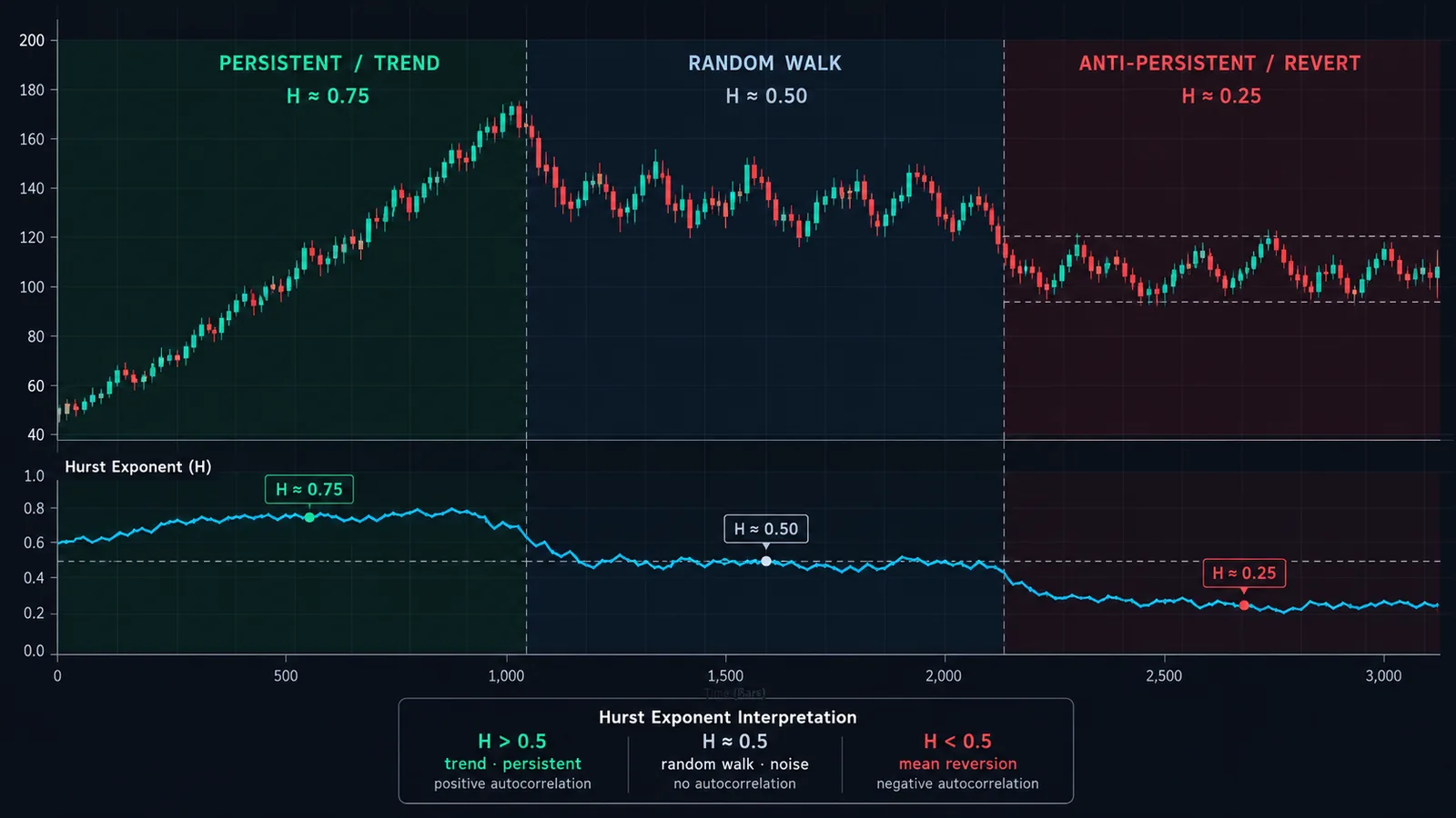
赫斯特指数 H 描述的是:当你观察一个累积序列越来越长的区间时,它的波动范围扩张得有多快。对收益率序列来说,它告诉你价格路径的波动区间随时间变宽的速度。重标极差大致遵循幂律关系:
(R/S)ₙ ≈ c × nᴴ
其中 n 为窗口长度。两边取对数后,H 就是 log(R/S) 对 log(n) 所拟合直线的斜率。
| H | 名称 | 对收益率意味着什么 | 适合的策略 |
|---|---|---|---|
| 低于 0.5 | 反持续性 | 上涨之后往往跟着下跌;价格路径不断折返 | 均值回归、逆向交易震荡指标极值、区间交易 |
| 约等于 0.5 | 随机游走 | 过去的走势无法提供下一步方向的任何信息 | 没有仅凭方向就能成立的策略 |
| 高于 0.5 | 持续性 | 走势倾向于延续;价格路径偏离起点的速度快于随机情况 | 趋势跟踪、通道突破、动量 |
有两点是大多数讲解都会略过的。
H is about returns, not prices. You feed the estimator the changes (log returns), and it studies how their cumulative sum, which is the price path, spreads out. Feed raw price levels into the same procedure and you get nonsense: in our tests, running R/S on the price levels of a pure random walk returned H of about 0.99, which says only that prices are prices.
H is not about drift. The R/S calculation subtracts the average return of each window before doing anything else. A market grinding steadily higher with choppy, back-and-forth daily returns can have H below 0.5. In a simulation of 200 random walks with and without a strong upward drift of 0.4% per bar, the corrected H was identical to three decimals. A steady trend in the everyday sense and persistence in the Hurst sense are different things. The second one is what matters for whether a trend-following rule will work.
你可能还会见到一个相关数值——分形维数,对自仿射序列而言 D = 2 − H。走势粗糙、锯齿状的均值回归图表,D 接近 2;走势平滑、具有持续性的图表,D 更接近 1。它包含的信息与 H 完全相同。
如何用 R/S 法逐步计算赫斯特指数
经典的重标极差(R/S)估算方法,按照 Hurst 的原始研究以及 Weron 等人后来的综述,对一个包含 L 个收益率的序列按如下步骤进行:
- Convert prices to log returns: rₜ = ln(Pₜ / Pₜ₋₁). Using logs keeps big and small price levels comparable.
- Pick window sizes. Choose several lengths n, usually doubling: 8, 16, 32, 64 and so on up to about L/2. Each needs at least two non-overlapping chunks.
- Split the series into L/n non-overlapping chunks of length n for each window size.
- Demean each chunk: subtract the chunk's average return from every return in it.
- Cumulate: build the running sum of the demeaned returns. This is the chunk's detrended price path.
- Range R: the maximum of the running sum minus the minimum.
- Scale S: the standard deviation of the chunk's returns.
- Rescale: compute R/S for the chunk, then average R/S across all chunks of the same length n.
- Regress: fit a straight line to log(average R/S) against log(n). The slope is the raw Hurst estimate.
- Correct for small-sample bias (optional but strongly recommended): subtract the R/S you would expect from pure noise at each n before fitting, then add 0.5. This is the Anis-Lloyd-Peters correction, covered below.
下文的计算器会对你粘贴的任何价格序列严格执行这十个步骤,并同时给出原始估计值和修正后的估计值。
实例演算:先手算一个数据块,再跑完整回归
第 1 步:单个 8 收益率数据块的 R/S
取八个以百分比表示的收益率:+1.0、+0.5、−0.8、+1.2、+0.3、−0.4、+0.9、+0.5。在 R/S 中单位会相互抵消,所以用百分比完全没问题。
| 收益率 | 减去均值(0.4) | 累计和 | 离差平方 |
|---|---|---|---|
| +1.0 | +0.6 | 0.6 | 0.36 |
| +0.5 | +0.1 | 0.7 | 0.01 |
| −0.8 | −1.2 | −0.5 | 1.44 |
| +1.2 | +0.8 | 0.3 | 0.64 |
| +0.3 | −0.1 | 0.2 | 0.01 |
| −0.4 | −0.8 | −0.6 | 0.64 |
| +0.9 | +0.5 | −0.1 | 0.25 |
| +0.5 | +0.1 | 0.0 | 0.01 |
The running sum peaks at 0.7 and bottoms at −0.6, so R = 1.3. The squared deviations total 3.36; divided by 8 that is 0.42, and the square root gives S = 0.648. So R/S = 1.3 / 0.648 = 2.006.
作为对比,根据 Anis-Lloyd 公式并加上 Peters 的调整,纯噪音在 8 个观测值上的 R/S 期望值是 2.461。这个数据块的游走幅度小于噪音。单个数据块几乎说明不了什么,这正是该方法要对大量数据块、多种窗口长度取平均的原因。
第 2 步:跨窗口长度的回归
下面在 256 个合成日收益率上完整跑一遍。这些数据由我们生成,带有轻微的短期动量(每天的收益率都带有前一天冲击的四分之一,即 φ = 0.25 的 AR(1) 过程):
| 窗口 n | 数据块数 | 平均 R/S | ln(n) | ln(R/S) | 期望 R/S(噪音) |
|---|---|---|---|---|---|
| 8 | 32 | 2.651 | 2.079 | 0.975 | 2.461 |
| 16 | 16 | 4.704 | 2.773 | 1.548 | 3.909 |
| 32 | 8 | 7.248 | 3.466 | 1.981 | 5.971 |
| 64 | 4 | 12.443 | 4.159 | 2.521 | 8.896 |
| 128 | 2 | 17.605 | 4.852 | 2.868 | 13.040 |
Fitting a least-squares line through the ln(n) and ln(R/S) columns gives a slope of 0.687. That is the raw Hurst exponent, and at face value it says "strongly trending".
Now fit the same line through the expected-noise column: its slope is 0.600. Pure randomness, measured over these particular windows, already produces a slope of 0.60, not 0.50. The corrected estimate is 0.5 + (0.687 − 0.600) = 0.587. Still persistent, but far less dramatic, and an honest reflection of the mild momentum we built in.
还要注意一点。我们模拟的过程只有短期记忆:每个收益率只依赖于前一天,与更早的数据无关。然而它依然把 H 推到了 0.5 以上。这正是 Andrew Lo 在 1991 年提出的问题,它对结果的解读至关重要,研究部分会详细说明。
为什么原始 R/S 会高估 H,以及 Anis-Lloyd 修正如何解决这一问题
经典 R/S 统计量在短样本中存在向上的偏差。Anis 和 Lloyd(1976 年,Biometrika 63(1): 111–116)推导出了独立正态观测值的重标极差期望值,Peters 后来又加入了一个小调整,改善了极短窗口下的表现。采用 Rafał Weron 在其 2002 年估算器精度研究中使用的形式:
E(R/S)ₙ = ((n − ½) / n) × Γ((n−1)/2) / (√π × Γ(n/2)) × Σᵢ₌₁ⁿ⁻¹ √((n − i) / i)
当 n > 340 时,将伽马函数之比替换为 1 / √(nπ/2)
修正后的赫斯特指数等于 0.5 加上 [log(R/S)ₙ − log E(R/S)ₙ] 对 log n 的斜率。换句话说:衡量你的序列比噪音扩散得快多少,再把这个差值加到噪音基准 0.5 上。
实际中这个偏差有多大?我们让 200 条模拟随机游走(真实 H = 0.5)通过同一个估算器,窗口从 8 开始:
| 样本长度(收益率个数) | 原始 R/S 的 H(平均值) | 修正后的 H(平均值) | 估计值离散度(1 个标准差) |
|---|---|---|---|
| 128 | 0.575 | 0.457 | ±0.076 |
| 256 | 0.568 | 0.468 | ±0.055 |
| 512 | 0.558 | 0.473 | ±0.044 |
| 1,024 | 0.559 | 0.485 | ±0.034 |
可以得出三个结论。
- Uncorrected R/S reads a coin flip as a mild trend. A raw H of 0.57 on a few hundred bars is exactly what pure randomness produces. Weron found the same: classical R/S "overestimates the true Hurst exponent to a great extent".
- The corrected version slightly undershoots. It comes in a little below 0.5 on short samples, a small negative bias Weron also reported for the corrected R/S, DFA and periodogram estimators.
- The error bars are wide. With 256 returns, one standard deviation of the estimate is about 0.055. A reading of 0.54 is noise. Weron also showed that the popular rule-of-thumb significance band of ±1/√L is too narrow and flags false positives too often.
Weron 的研究在修正 R/S 时只使用长度大于 50 的窗口,因为纳入极短窗口会放大方差。这需要数千根 K 线。只有几百根 K 线的交易者通常只能接受短窗口,也就应当接受随之而来的更宽误差范围。
R/S 的替代方法:DFA、方差比与聚合方差
R/S 是最早的方法,但不是最好的。下面是你最常遇到的几种估算方法:
| 方法 | 思路 | 优点 | 缺点 |
|---|---|---|---|
| 重标极差(R/S) | 累计离差的极差除以标准差,再对窗口长度做回归 | 简单、历史悠久、直观 | 小样本中有偏;对短期自相关敏感 |
| 去趋势波动分析(DFA) | 在累积序列的每个窗口内拟合局部趋势线,度量剩余波动 F(n),取 log F 对 log n 的斜率 | 在 Weron 的测试中,短样本上精度最高;能容忍缓慢的趋势 | 计算量更大;没有闭式分布 |
| 方差比 | q 根 K 线收益率的方差除以 q 倍的单根 K 线收益率方差;大于 1 表示持续性,小于 1 表示均值回归 | 有正式的统计检验(Lo 与 MacKinlay,1988) | 一次只能检验一个周期 |
| 聚合方差 | 随着分块大小 m 增大,分块均值的方差按 m^(2H−2) 缩小 | 计算简单 | 噪音大;容易被趋势和水平位移干扰 |
| 周期图法(GPH) | 频谱低频端的斜率 | 渐近理论成熟 | 需要长样本 |
DFA 由 Peng 及其同事于 1994 年在一项 DNA 序列研究中提出(Physical Review E 49: 1685–1689),如今已是物理学和经济物理学文献中的默认方法。Weron 在模拟白噪音上做的对比中,称 DFA 是他所测试的三种方法中“无可争议的赢家”。如果你在搭建自己的市场状态过滤器,并且不介意多写几行代码,就用 DFA,把 R/S 留作交叉验证。如果你的目标是更干净地估计潜在趋势,而不是给市场状态贴标签,那么像卡尔曼滤波这样的状态空间方法能更直接地回答这个问题。
方差比值得了解,则是出于另一个原因。Lo 和 MacKinlay 在《Stock Market Prices Do Not Follow Random Walks》(Review of Financial Studies,1988)中使用了它,对 1962 年至 1985 年美国股票周收益率强烈拒绝了随机游走假设,而这一拒绝主要由小盘股驱动。它检验的是某个特定周期,这与交易者的思维方式相契合:“5 天的走势是否有持续性?”正是一个方差比问题。
赫斯特指数在市场中有效吗?研究怎么说
证据确实存在,但适用范围比交易博客里描述的要窄。
- Short memory masquerading as long memory. Andrew Lo's "Long-Term Memory in Stock Market Prices" (Econometrica, 1991, 59(5): 1279–1313) built a modified R/S test that allows for short-range dependence. Applied to daily and monthly US stock indexes, it found no evidence of long-range dependence once short-term autocorrelation was accounted for, contrary to earlier claims based on classical R/S. Our worked example shows the mechanism: one day of momentum is enough to lift the classical estimate above 0.5.
- Hurst and predictability across markets. Eom, Choi, Oh and Jung studied 60 market indexes and found a strong positive relationship between each index's Hurst exponent and the hit rate of a nearest-neighbour forecast of price direction. Markets with higher H were more predictable, and the authors suggested the measure helps separate emerging from mature markets.
- Strategy switching. Chang, Lizardi and Shah (2022) used the Hurst exponent to choose between momentum and mean-reversion strategies and reported that the Hurst-based approach could achieve higher returns, though with higher risk.
- Estimator accuracy. Weron (2002) showed how wide the confidence intervals are on realistic sample sizes and that DFA is the most reliable of the common estimators.
综合来看:大型、高流动性市场的日收益率接近 0.5,所谓的长期记忆往往其实是短期自相关或波动率效应。但这并不意味着 H 对交易者毫无用处。短期持续性恰恰是趋势跟踪规则所利用的东西;一个在持续性出现时上升、在收益率开始反转时下降的指标,即使计量经济学家不会称之为长期记忆,也依然有用。只是别把 0.58 的读数当成什么重大发现。
把滚动赫斯特指数用作市场状态过滤器
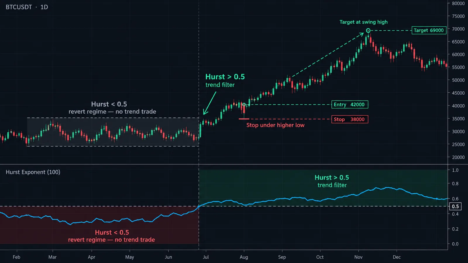
赫斯特指数在交易中最实用的用法不是预测价格,而是决定运行哪一类策略。滚动赫斯特指数在每根 K 线上用最近一个窗口的收益率重新计算,充当趋势跟踪与均值回归两套打法之间的切换开关。
一个具体的设计方案
- Window: 256 daily returns (about a year) on the instrument you trade, or 256 four-hour bars for a faster read. Shorter windows react quicker but the error bars widen fast.
- Estimator: corrected R/S or DFA, windows 8 to 128. Never the raw R/S slope, which is biased upward by about 0.07 at this length.
- Noise band: with 256 returns, readings within about ±0.05 of 0.5 are indistinguishable from randomness. A simple rule: band = 0.85 / √L, which is roughly one standard deviation in our simulations.
- Regimes: H above 0.55 = trend regime; below 0.45 = mean-reversion regime; anything between = stand aside or trade smaller.
- Hysteresis: enter a regime when H crosses the band edge, exit only when it crosses back through 0.5. That stops the switch from flickering every few bars.
- Smoothing: a short average (5 to 10 bars) of the rolling H reduces noise further, at the cost of a few bars' delay.
各市场状态下运行什么策略
- Trend regime: breakouts and moving-average systems such as an ALMA crossover or a McGinley Dynamic trend line, with trailing exits.
- Mean-reversion regime: fades of band extremes using Bollinger Bands or RSI extremes, with fixed targets near the mean. Our mean reversion trading guide covers rules for this side.
- Neutral: reduced size, or nothing.
同样的思路也适用于配对和价差交易。赫斯特指数持续偏低的价差是均值回归交易的候选对象;而 H 向 0.5 甚至更高攀升的价差,正在失去让它可交易的那种特性。
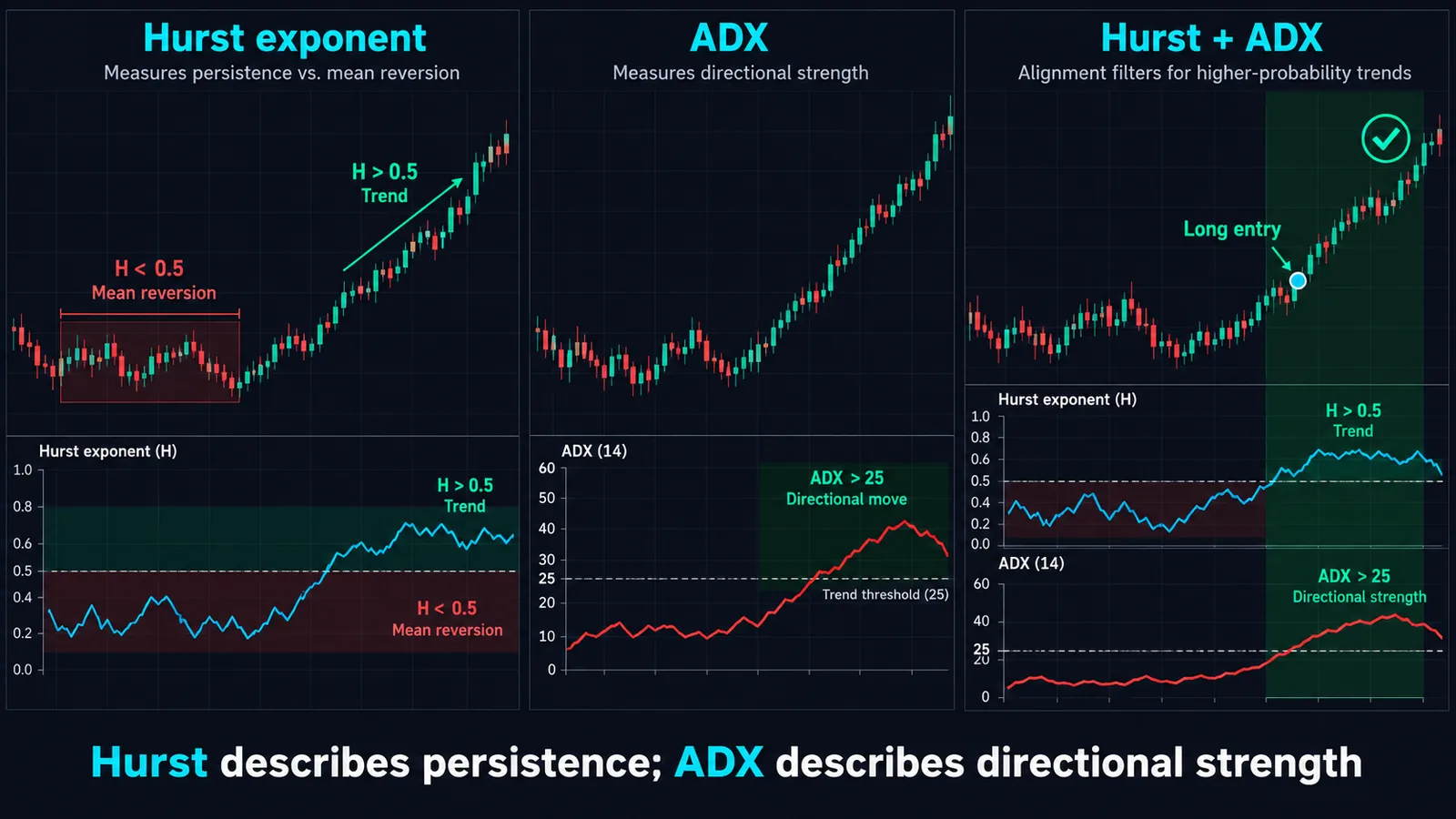
如果你想要一个不依赖收益率统计的第二意见,ADX 根据价格区间衡量趋势强度,可以作为很有用的交叉验证;两者在拐点处经常给出不同结论,而这种分歧本身就是信息。
TradingView 上有赫斯特指数指标吗?
据我们所知,TradingView 的内置指标中并没有赫斯特指数。社区脚本库里有不少开源脚本可以估算它,通常以震荡指标的形式绘制在独立的副图中,并带有一条 0.5 参考线。在“指标”对话框中搜索“Hurst”,然后筛选社区脚本即可。
在信任任何一个脚本之前,先打开源代码检查以下五点:
- Returns or prices? The estimator must run on returns (ideally log returns). A script that feeds price levels into R/S will sit near 1.0 forever.
- Raw or corrected? If the script fits log(R/S) without subtracting the expected noise value, subtract roughly 0.05 to 0.10 from its readings in your head on typical lookbacks.
- Window sizes. At least three or four sizes should go into the regression. A "Hurst" computed from a single window is just a scaled range, not an exponent.
- Lookback. Under about 100 bars, the estimate is too noisy to separate 0.45 from 0.55 reliably.
- Repainting. A proper rolling estimate only uses closed bars. If historical values shift when you reload the chart, see our non-repaint indicators guide.
给 Pine 作者的一个实用提示:在每根 K 线上对多个窗口长度计算 R/S 会涉及嵌套循环,回看周期较长时可能触及 Pine 的执行限制。如果你只需要当前的市场状态,可以只在最后一根 K 线上计算,或每隔 N 根 K 线计算一次。平台基础知识请参阅我们的 TradingView 平台指南。要检验任何脚本是否靠谱,可以导出或复制几百个收盘价粘贴到本页的计算器中进行对比。
常见错误,以及赫斯特指数何时会误导你
- Reading raw R/S at face value. On a few hundred bars, raw R/S averages about 0.57 on pure noise. Use the corrected version or DFA.
- Ignoring the error bars. With 256 returns, ±0.055 is one standard deviation. Regime calls inside 0.45 to 0.55 are guesses.
- Confusing short and long memory. One day of momentum lifts H. That may be tradable, but it decays quickly; don't extrapolate it to multi-month horizons.
- Non-stationary samples. A window that contains a crash and a calm recovery mixes two regimes. Volatility clustering itself had little effect in our simulations, but structural breaks, such as a policy change, a halving cycle in crypto, or a product rolling from one contract to another, can distort the estimate badly. Use back-adjusted continuous contracts for futures.
- Mixing timeframes. H on 5-minute returns and H on daily returns answer different questions and can point opposite ways, so measure it on the timeframe you actually trade, whether that is daily swings or scalping charts. Microstructure effects such as the bid-ask bounce push very short-timeframe returns toward mean reversion.
- Calling drift persistence. A strong uptrend with choppy returns can read 0.5 or lower. If you need a trend-in-price measure, use slope-based tools such as a linear regression channel alongside H.
- Optimizing the threshold. Choosing 0.53 because it maximized a backtest is data snooping. Set the band from sample size, not from results.
- Too few window sizes. Two points always fit a line perfectly. Use at least three, preferably four or more.
赫斯特指数与 Quantum Algo
赫斯特指数回答的是一个大多数指标从不关心的问题:这个市场眼下奖励的是趋势跟踪,还是逆向交易?这使它成为一个过滤器,而不是触发信号。它告诉你该拿起哪些工具,而不是什么时候按下按钮。
一种可行的分工方式:用你所交易品种上滚动的、经过修正的赫斯特指数来确定市场状态;在趋势状态下,由信号工具负责把握时机。在 QuantumAlgo 的 Zeno 套件中,这意味着当市场状态显示为持续性时,更积极地采纳 Zeno 的买卖信号(信号自带止损和目标位);当显示为反持续性时,则选择观望或减小仓位。你可以在公开的历史业绩记录中自行评估这些信号的表现。在均值回归状态下,我们的免费Market Bottom Finder和Multi-Oscillator Divergence Scanner更适合这项工作,而 Event Probability Engine 则适合已经习惯用概率思考的交易者。
在统计层面,相关的机器学习指标指南介绍了其他判别市场状态的方法,免费的Academy则帮你打好趋势与均值回归的基础——这两种市场状态都离不开这些基础。
◆ 互动检查
您对 赫斯特指数 了解多少?
交易者常问的 赫斯特指数 问题
它是一个介于 0 到 1 之间的数值,描述收益率倾向于延续还是反转。高于 0.5 表示趋势行为,约等于 0.5 表示随机游走,低于 0.5 表示均值回归。交易者主要用它来判断哪种策略适合当前的市场环境。
经典方法是重标极差分析:把对数收益率切分成若干种长度的数据块,对每个数据块计算累计离差的极差除以标准差,按长度取平均,再求 log(R/S) 对 log(长度) 的斜率。样本较短时,还要用噪音的 R/S 期望值对结果进行修正。
没有好坏之分,只有合不合适。趋势策略需要明显高于 0.5 的读数,均值回归策略需要明显低于 0.5 的读数。如果只有几百根 K 线,大约 0.45 到 0.55 之间的数值都应视为随机。
英国水文学家 Harold Edwin Hurst,他在研究尼罗河流量以确定水库规模时提出了这一概念,并于 1951 年发表了重标极差方法。Benoit Mandelbrot 后来拓展了这一思想,并将其应用于金融市场。
这意味着收益率表现得像随机游走:过去的方向对未来的方向毫无提示作用。在短样本上,由于存在偏差,未修正的估计值即使为 0.55 到 0.58,也可能与随机游走一致。
要得到可用于交易的估计值,至少需要几百个收益率;要达到研究级精度,则需要数千个。在我们的模拟中,256 个收益率下估计值的一个标准差约为 0.05。
通常是的。在 Weron 2002 年基于模拟数据的对比中,去趋势波动分析是所测试方法中最准确的。R/S 仍然可以作为一种简单的交叉验证手段。
据我们所知没有内置指标,但有几个社区脚本可以估算它。在信任某个脚本之前,先确认它使用的是收益率、做了偏差修正,并且对多个窗口长度进行了回归。
不能。它描述的是近期收益率的特性,而不是下一步往哪个方向走。Eom 等人对 60 个指数的研究等成果表明,H 越高,可预测性越好,但方向判断仍然要靠你自己的策略。
它是独立正态数据的重标极差期望值,由 Anis 和 Lloyd 于 1976 年推导得出,后经 Peters 改进。在每个窗口长度上从观测到的 R/S 中减去它,就能消除经典估算器的大部分向上偏差。
参考资料与相关指南
接下来阅读
- 均值回归交易:完整策略指南
- ADX 指标 (Average Directional Index)
- 机器学习交易指标
- Bollinger Bands:完整交易指标指南
- 线性回归通道:如何绘制、解读和交易
- Kaufman 自适应移动平均线(KAMA):懂得何时停止移动的平均线
- 免费 TradingView 指标
- Zeno — 高级引擎
主要来源
- Wikipedia — Hurst exponent
- Wikipedia — Harold Edwin Hurst
- Weron (2002) — Estimating long range dependence: finite sample properties and confidence intervals (arXiv)
- Econometric Society — Lo (1991), Long-Term Memory in Stock Market Prices, Econometrica 59(5)
- MIT — Lo & MacKinlay (1988), Stock Market Prices Do Not Follow Random Walks
- Eom, Choi, Oh & Jung — Hurst exponent and prediction based on weak-form efficient market hypothesis (arXiv)
- Chang, Lizardi & Shah (2022) — Optimizing Returns Using the Hurst Exponent and Q Learning (arXiv)
- Wikipedia — Detrended fluctuation analysis